File:Gradient descent.svg

Dimensioni di questa anteprima PNG per questo file SVG: 512 × 549 pixel. Altre risoluzioni: 224 × 240 pixel | 448 × 480 pixel | 716 × 768 pixel | 955 × 1 024 pixel | 1 910 × 2 048 pixel.
File originale (file in formato SVG, dimensioni nominali 512 × 549 pixel, dimensione del file: 56 KB)
| Questo file e la sua pagina di descrizione (discussione · modifica) si trovano su Wikimedia Commons (?) |
Dettagli
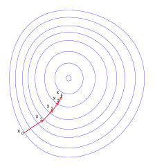
| Descrizione | An illustration of the gradient descent method. I graphed this with Matlab |
| Data | (UTC) |
| Fonte |
Questo file deriva da: Gradient descent.png:  |
| Autore |
|
| Questa è una immagine ritoccata, il che significa che è stata modificata digitalmente dalla sua versione originale. Modifiche: Vector version. La versione originale può essere vista qui: Gradient descent.png. Le modifiche sono di Zerodamage.
|
Licenza
Io, detentore del copyright su quest'opera, dichiaro di pubblicarla con la seguente licenza:
| Io, detentore del copyright su quest'opera, la rilascio nel pubblico dominio. Questa norma si applica in tutto il mondo. In alcuni paesi questo potrebbe non essere legalmente possibile. In tal caso: Garantisco a chiunque il diritto di utilizzare quest'opera per qualsiasi scopo, senza alcuna condizione, a meno che tali condizioni siano richieste dalla legge. |
Source code
% Illustration of gradient descent
function main()

% the ploting window
   figure(1);
   clf; hold on;
   set(gcf, 'color', 'white');
   set(gcf, 'InvertHardCopy', 'off');
   axis equal; axis off;

% the box
   Lx1=-2; Lx2=2; Ly1=-2; Ly2=2;

% the function whose contours will be plotted
   N=60; h=1/N;
   XX=Lx1:h:Lx2;
   YY=Ly1:h:Ly2;
   [X, Y]=meshgrid(XX, YY);
   f=inline('-((y+1).^4/25+(x-1).^4/10+x.^2+y.^2-1)');
   Z=f(X, Y);

% the contours
   h=0.3; l0=-1; l1=20;
   l0=h*floor(l0/h);
   l1=h*floor(l1/h);
   v=[l0:1.5*h:0 0:h:l1 0.8 0.888];
   [c,h] = contour(X, Y, Z, v, 'b');

% graphing settings
   small=0.08;
   small_rad = 0.01;
   thickness=1; arrowsize=0.06; arrow_type=2;
   fontsize=13;
   red = [1, 0, 0];
   white = 0.99*[1, 1, 1];

% initial guess for gradient descent
   x=-0.6498; y=-1.0212;

   % run several iterations of gradient descent
   for i=0:4
      H=text(x-1.5*small, y+small/2, sprintf('x_%d', i));
      set(H, 'fontsize', fontsize, 'color', 0*[1 1 1]);

     % the derivatives in x and in y, the step size
      u=-2/5*(x-1)^3-2*x;
      v=-4/25*(y+1)^3-2*y;
      alpha=0.11;

      if i< 4
         plot([x, x+alpha*u], [y, y+alpha*v]);
         arrow([x, y], [x, y]+alpha*[u, v], thickness, arrowsize, pi/8, ...
               arrow_type, [1, 0, 0])
         x=x+alpha*u; y=y+alpha*v;
      end

   end

% some dummy text, to expand the saving window a bit
   text(-0.9721, -1.5101, '*', 'color', white);
   text(1.5235,   1.1824, '*', 'color', white);

% save to eps
   saveas(gcf, 'Gradient_descent.eps', 'psc2')

function arrow(start, stop, thickness, arrow_size, sharpness, arrow_type, color)

% Function arguments:
% start, stop:  start and end coordinates of arrow, vectors of size 2
% thickness:    thickness of arrow stick
% arrow_size:   the size of the two sides of the angle in this picture ->
% sharpness:    angle between the arrow stick and arrow side, in radians
% arrow_type:   1 for filled arrow, otherwise the arrow will be just two segments
% color:        arrow color, a vector of length three with values in [0, 1]

% convert to complex numbers
   i=sqrt(-1);
   start=start(1)+i*start(2); stop=stop(1)+i*stop(2);
   rotate_angle=exp(i*sharpness);

% points making up the arrow tip (besides the "stop" point)
   point1 = stop - (arrow_size*rotate_angle)*(stop-start)/abs(stop-start);
   point2 = stop - (arrow_size/rotate_angle)*(stop-start)/abs(stop-start);

   if arrow_type==1 % filled arrow

% plot the stick, but not till the end, looks bad
      t=0.5*arrow_size*cos(sharpness)/abs(stop-start); stop1=t*start+(1-t)*stop;
      plot(real([start, stop1]), imag([start, stop1]), 'LineWidth', thickness, 'Color', color);

% fill the arrow
      H=fill(real([stop, point1, point2]), imag([stop, point1, point2]), color);
      set(H, 'EdgeColor', 'none')

   else % two-segment arrow
      plot(real([start, stop]), imag([start, stop]),   'LineWidth', thickness, 'Color', color);
      plot(real([stop, point1]), imag([stop, point1]), 'LineWidth', thickness, 'Color', color);
      plot(real([stop, point2]), imag([stop, point2]), 'LineWidth', thickness, 'Color', color);
   end

function ball(x, y, r, color)
   Theta=0:0.1:2*pi;
   X=r*cos(Theta)+x;
   Y=r*sin(Theta)+y;
   H=fill(X, Y, color);
   set(H, 'EdgeColor', 'none');

%plot2svg must be retrieved from http://www.zhinst.com/blogs/schwizer/
plot2svg;
Registro originale del caricamento
This image is a derivative work of the following images:
- File:Gradient_descent.png licensed with PD-self
- 2007-06-23T03:33:09Z Oleg Alexandrov 482x529 (25564 Bytes) {{Information |Description=An illustration of the gradient descent method. I graphed this with Matlab |Source=Originally from [http://en.wikipedia.org en.wikipedia]; description page is/was [http://en.wikipedia.org/w/index.ph
Uploaded with derivativeFX
Cronologia del file
Fare clic su un gruppo data/ora per vedere il file come si presentava nel momento indicato.
| Data/Ora | Miniatura | Dimensioni | Utente | Commento | |
|---|---|---|---|---|---|
| attuale | 21:04, 7 ago 2012 | | 512 × 549 (56 KB) | Zerodamage | == {{int:filedesc}} == {{Information |Description=An illustration of the gradient descent method. I graphed this with Matlab |Source={{Derived from|Gradient_descent.png|display=50}} |Date=2012-08-07 19:02 (UTC) |Author=*File:Gradient_descent.png:... |
Pagine che usano questo file
La seguente pagina usa questo file:
Utilizzo globale del file
Anche i seguenti wiki usano questo file:
- Usato nelle seguenti pagine di ar.wikipedia.org:
- Usato nelle seguenti pagine di ca.wikipedia.org:
- Usato nelle seguenti pagine di cs.wikipedia.org:
- Usato nelle seguenti pagine di de.wikiversity.org:
- Usato nelle seguenti pagine di en.wikipedia.org:
- Usato nelle seguenti pagine di en.wikiversity.org:
- Usato nelle seguenti pagine di he.wikipedia.org:
- Usato nelle seguenti pagine di pt.wikipedia.org:
- Usato nelle seguenti pagine di sr.wikipedia.org:
- Usato nelle seguenti pagine di uk.wikipedia.org:
- Usato nelle seguenti pagine di vi.wikipedia.org:
- Usato nelle seguenti pagine di zh-yue.wikipedia.org: